Paper Summary: Making Gradient Descent Optimal for Strongly Convex Stochastic Optimization
In this blog, I will give a summary of the paper “Making Gradient Descent Optimal for Strongly Convex Stochastic Optimization” and some of my understandings. A full version with proofs can be found at arxiv. For stardard stochastic gradient descent (SGD) method with strongly convex problem, the convergence rate is known to be \(O(log(T)/T)\), while there are other algorithms achieves \(O(1/T)\) convergence rate. Is \(O(log(T)/T)\) a tight bound for SGD? In this paper, the authors give an example of strongly convex and non-smooth problem where the stardard stochastic gradient descent (SGD) has a \(\Omega(log(T)/T)\). This justify the claim that \(O(log(T)/T)\) is a tight bound for stardard SGD. Moreover, a simple modification of SGD is shown to be sufficient to recover the \(O(1/T)\) rate.
1. Stochastic Gradient Descent
Stochastic Gradient Descent (SGD) is a well-known and popular method to solve a convex stochastic optimization problem. The goal is to minimize the objective \(F\) over some convex domain \(W\), without the knowledge of \(F\). The only information we can obtain is a stochastic gradient oracle. For each input \(w\in W\), the oracle will output a vector \(\hat{g}\) whose expectation \(E(\hat{g}) = g \in \partial F(w)\) is a subgradient of \(F\) at \(w\).
In SGD method, we first arbitrarily select a initial point \(w\) inside the convex domain \(W\). Then at each iteration step \(t=1,\dots,T\), we call the stochastic gradient oracle to obtain the \(\hat{g}_t\), then update the optimization variable by
\[w_{t+1} = \Pi_{W}(w_t-\eta_t \hat{g}_t)\]Here, the step size \(\eta_t\) is designed by users. \(\Pi_{W}\) is the projection operator on the convex domain \(W\). After getting the sequence of points \(w_1,\dots,w_T\), stardard SGD returns the average point
\[\bar{w}_T = \frac{1}{T}(w_1+\dots+w_T)\]For \(\lambda\)-strongly convex function \(F\), the authors consider the general step sizes \(\eta_t = {c}/({\lambda t})\) and it can be shown that the step size of \(\Theta(1/t)\) is necessary to obtain the optimal convergence rate. For smooth problem, the last point of SGD converges with \(O(1/T)\). Mathemcatically, suppose \(F\) is \(\lambda\)-stronly convex and \(\mu\)-smooth with repect to the optimal point \(w^*\), and suppose \(E[|| \hat{g}_t||^2] \leq G^2\). Then with step size \(\eta_t = c/(\lambda t)\) and \(c>1/2\), we have:
\[E[F(W_T)-F(w^*)] \leq \frac{1}{2}max\{ 4,\; \frac{c}{2-1/c} \} \frac{\mu G^2}{\lambda^2 T}\]This inequality claims that the expected difference between the objective at last point \(F(w_T)\) and optimal value \(F(w^*)\) is at most order of \((1/T)\). For the average point \(\bar{w}_T\), it also enjoys an \(O(1/T)\) rate.
2. Non-Smooth Problems
So far, SGD works well with stronly convex and smooth objective functions. But what about non-smooth functions? In the literature, SGD with averaging is known to have a \(O(log(T)/T)\). Besides, there are other optimal algorithms that achieve \(O(1/T)\). One natural question to ask is what makes this gap. Is it because of the property of SGD or the loose analysis? In the paper, the authors give a simple example, on which SGD with averaging has a \(\Omega(log(T)/T)\). This actually shows that the convergence rate \(O(log(T)/T)\) is tight. The example is given as follows. Let \(F\) be the function:
\[F(w) = \frac{1}{2} ||w||^2 + w_1\]where the domain \(W=[0,1]^d\). Upon enquries, the gradient oracle produces the estimate \(\hat{g}_t = w_t + (Z_t,0,\dots,0)\). The random variable \(Z_t\) is uniformly distributed over \([-1,3]\). As claimed in theorem 3, there exist a \(T_0\) such that the following inequality holds for any \(T \geq T_0 + 1\).
\[E[F(\bar{w}_T)-F(w^*)] \geq \frac{c}{16T} \sum_{t=T_0}^{T-1} \frac{1}{t}\]Therefore, the lower bound of SGD with averaging is \(\Omega(log(T)/T)\). The intuition behind this example is that the non-smooth function \(F\) is designed such that the iterates \(w_t\) appoach the optimum from just one direction. This example shows that the convergence rate \(O(log(T)/T)\) is indeeed tight for SGD with averaging, which is the property of this method.
3. SGD with \(\alpha\)-Suffix Averaging
In the literature, there are some algorithms that achieve the optimal \(O(1/T)\) rate for any \(F\). But those algorithms are complicated and different from the idea of SGD. This paper gives a rather simple modification to standard SGD. Instead of averaging all the iterates \(w_t\), the modified version focus on last \(\alpha\)-proportion of \(T\) iterations. In particular, given a constant \(\alpha \in (0,1)\), the returned value is given by:
\[\bar{w}^{\alpha}_T = \frac{w_{(1-\alpha)T+1}+\dots+w_T}{\alpha T}\]where we assume \(\alpha T\) and \((1-\alpha)T\) are integers. This method is called \(\alpha\)-suffix averaging. As claimed in theorem 5, the expected difference is bounded by the following inequality:
\[E[F(\bar{w}_T^{\alpha})-F(w^*)] \leq c_0 \cdot \frac{log(\frac{1}{1-\alpha})}{\alpha} \cdot \frac{G^2}{\lambda T}\]where \(c_0\) is a constant factor that only depends on \(c\). And for any \(\alpha \in (0,1)\), the bound is \(O(G^2/\lambda T)\) which approaches the optimal guarantees up to constant factors. The table below summaries the convergence rate for the different methods and different assumptions discussed in the paper. In the table, SGD-A is standard SGD with averaging, SGD-\(\alpha\) is SGD with \(\alpha\)-suffix averaging as discussed in this section, EPOCH-GD is the optimal algorithm proposed in [1].
| strongly convex | non-smooth | rate | |
|---|---|---|---|
| SGD-A | ☑ | ☒ | \(O(1/T)\) |
| ☑ | ☑ | \(O(log(T)/T)\) | |
| SGD-\(\alpha\) | ☑ | ☑ | \(O(1/T)\) |
| EPOCH-GD | ☑ | ☑ | \(O(1/T)\) |
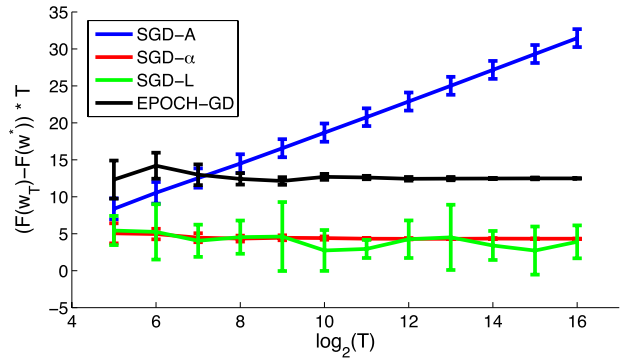
Besides, the figure below (figure 2 in the original paper) shows the experiment results of different algorithms in example constructed in the previous section. The additional SGD-L plot is for SGD return with last iterate. We can observe from the figure that the SGD-A (blue line) indeed suffers from a \(O(log(T)/T)\) tight bound in this example.
4. Conclusion
This paper shows the tight bound of standard SGD by an example. The SGD with \(\alpha\)-suffix averaging is proposed to close the gap between standard SGD and the optimal algorithm. The numerical results valid the theoretical analysis. I really enjoy reading this paper since everything is clearly addressed.
References
[1] Hazan, E. and Kale, S. Beyond the regret minimization barrier: An optimal algorithm for stochastic strongly-convex optimization. In COLT, 2011.